Lab 4
Sampling Efficiency
Due: Thursday, December 15th, 2016, 23:59
This lab was modeled after the assignment 4 of Stanford's Image Synthesis class.- Individual Effort:
- No team participation is really encouraged in the case of the homework or the labs.
- Late Submission:
- In general late submission is not encouraged/accepted unless
there is a very good reason. You are encouraged to submit on time. We
are on a tight schedule. Being late for one lab could affect the time
left for you to complete subsequent labs. Late Submissions are
possible, yet they will be penalized.
- One day late: 15% penalty
- Two days late: 30% penalty
- Three days late: 50% penalty
- Four or more days late: 100% penalty.
Objectives
In this assignment you will evaluate the efficiency of different sampling strategies for Monte-Carlo integration. While there is very little coding in this assignment, you will probably need to script pbrt to collect the right data. The data collection itself may take some time, so plan ahead to make sure you have time to complete rendering. You can download the necessary scene files and reference images.
Sampling and Variance
Variance of a random variable X is defined as E[ (X - E[X])^2 ]. To compute the variance of an image rendered by pbrt we can compare it, pixel by pixel, to a reference image that we consider to be ground truth for E[X]. We've included three EXR images that will serve as ground truth for this assignment (occluder_ref.exr, occluder_shadow_ref.exr, and manykilleroos_ref.exr). These scenes were rendered with 16384 samples per pixel to ensure that they are very close to the correct image. To measure the variance of any image you render, you can use the exrdiff program that is included with pbrt:exrdiff image_ref.exr yourimage.exrThis will print something like:
Images differ: 173884 big (64.40%), 179244 small (66.39%)
avg 1 = 0.351801, avg2 = 0.361679 (-2.807667% delta)
MSE = 0.126821
Look at the code for exrdiff and convince yourself that the MSE (mean-squared error) value it calculates is equivalent to the variance. You may need to modify exrdiff to ensure it always prints the MSE value regardless of how close the two images are.
As we increase the number of samples taken, we expect the the variance to go down. We will measure this change empirically by modifying the pixelsamples variable in the scene files. The file occluder.pbrt contains a scene with a single area-light, a square occluder, and a large ground plane:
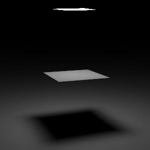
Render this scene varying the number of samples from 1 to 64, and compute the variance of each image. You only need to measure powers of 2 since many of the samplers in pbrt will round this number to a power of 2 anyway.
The scene file is setup to use a low-discrepancy sampler which tries to generate well-distributed non-uniform points such that no two points are close together. Let's compare this to a purely random sampler, by changing "lowdiscrepancy" to "random" in the scene file, and finding the variance for each image.
Deliverables
First, submit a graph showing the variance for both the random and low-discrepancy samplers as you increase pixelsamples from 1 to 64 for theoccluder.pbrt scene. You will probably want to use log scale for both axes since you are only considering powers of 2. Furthermore, you should answer the following questions:
Question 1. When using Monte-Carlo sampling with uniformly sampled random variables, how does the variance change as a function of the number of samples taken, N? Does the data you collected reflect this behavior?
Question 2. How does the low-discrepancy sampler perform in comparison to random sampling? Why does distributing the samples evenly through space change the variance in comparison to random sampling?
Evaluating Efficiency
In lecture, we discussed different strategies for sampling the value for a pixel. In one variation, we compute an intersection with the scene and a ray, and then evaluate the radiance along the ray using N samples from each area light. In another variation, rather than taking multiple samples, we take only a single sample (N = 1), and compensate by increasing the number of samples taken per pixel.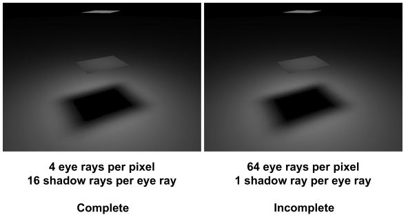
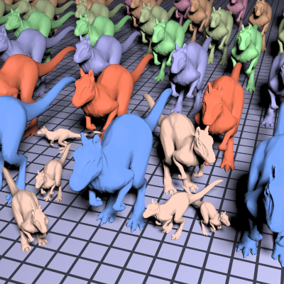
Your task for this step is to compare the efficiency of these approaches on the three scenes we have included: occluder.pbrt, occluder_shadow.pbrt (a different view of the first scene), and manykilleroos.pbrt:

You should consider strategies from N=1 sample per light to N = 64 samples, again in powers of 2. One strategy is considered more efficient than another if, given a fixed amount of time, it can compute an image with less variance than the image produced by the other strategy (alternatively, given a target variance, it is more efficient if it can compute the image in less time).
Evaluate each strategy (1 to 64 samples per light) by rendering images for a range of pixelsamples (1 to 64 samples per pixel). For each image, you should measure the amount of time it takes to render, as well as the variance of the result. To limit the number of scenes you have to render, you can limit yourself to scenes where the [number of light samples] x [number of pixel samples] <= 64. You should only time the rendering of the scene, not the setup costs. This is particular important for the manykilleroo scene, which has complex geometry.
Deliverables
For each scene, you should construct a graph that compares the efficiencies of the different strategies, and explain what the graph is showing. Furthermore, you should answer the following questions.Question 1. For each scene, which approach(s) (e.g 1 light sample per pixel sample, 2 light samples per pixel sample, ...) perform(s) most efficiently. Why do you think that is the case? Backup your answer using data from the graphs you have generated.
Question 2. Is the same approach best across all the scenes? Why or why not? Are any approaches particularly bad? Why?
Question 3. What characteristics in the scene make the path tracing (N=1) method more efficient? What characteristics make strategies with a large number of light samples more efficient?
Final Project
At this time you should be finalizing your final project plans. I.e. I would like to see a detailed writeup on:- The method: What exactly are you trying to achieve and how? Your writeup should not be shy of details, explain the proper previous work you are relying on and describe exactly on how you will make it all work.
- The milestones: Include a description of each project milestone with start / end dates and who will be assigned to accomplish each milestone. These should be detailed enough that you know if the amount of work you are proposing is reasonable.
- Implementation details: A brief description of the language, platform, and any toolkit(s) you plan to use, and reasons for these choices.
Submission
Please submit your answers in a single PDF file in moodle, in Lab4 section
here.
If you have multiple files to upload (e.g. source code or supplementary pictures),
please upload all your submission as a single compressed ZIP file.
We expect a good student to have to work approximately 10 hours on this assignment.
Include one paragraph about your estimated effort you put into this lab. How many (focused) hours of work did it take you and roughly where did you spend most of your time.
Grading
This assignment will be graded on a 5 point scale:
- 1 point: A writeup with majors errors.
- 2 points: A correct writeup but step 1 or step 2 is incomplete.
- 3 points: A complete writeup with but explanations are not clear, or contain minor errors.
- 4 points: A correct, clear, and complete writeup
- the fifth point is for the proper writeup and progress report for the final project.