Lab 3
Light Field Camera
Due: Thu, December 14 2017, 23:59
Start Early!!!
This lab was modeled after the assignment 3 of Stanford's Image Synthesis class.Light field cameras allow user to capture a 4-dimensional radiance (Light Field) and then use it to synthesize new images with different camera settings by sampling and reconstructing form the light field.
PBRT comes with four built-in cameras: Simple Orthographic and Perspective thin lens models,
Environment camera for full 360 degree view, and Realistic camera with data-driven lens system. You
will be extending pbrt to include a light field camera, and then extending
imgtool to synthesize images using the produced light field.
Step 1: Background Reading
Light fields has been introduced to the graphics literature in 1996 by Levoy and Hanrahan in a SIGGRAPH paper Light Field Rendering. It involves prefiltering the light field before sampling to avoid aliasing, at the expense of only being able to re-render a shallow depth-of-field.
This lab exercise is based on a follow up paper form 2000, Dynamically Reparameterized Light Field with the focus of being able to moderately sample scenes with a wide depth range into a light field, and reconstruct images with widely varying aperture setting and focal planes, even allowing non-planar focal planes.
Step 2: Extend PBRT with Light Field Camera
You will be extending PBRT to have a new camera subclass. The new camera should simulate a 2D array of equally spaced pinhole cameras, called data cameras, with identical resolution and field of view. This configuration is a restricted subset of the configuration in the Dynamically Reparameterized Light Field paper. The lab3_scenes set provides a set of useful scenes for testing your code and submit your results.
To add a new camera, you need to follow the same procedure as lab-2. Create two new files
lightfield.h and lightfield.cpp, which include the code for the new
camera subclass. Provide a CreateLightFieldCamera(...) to prepare the camera and
call it form api.cpp, where the camera parameters are parsed and camera instances
are created. You should parse "shutteropen", "shutterclose" and "fov" in the
same way perspective camera does. Further, you should accept the parameters "camerasperdim"
and "cameragridbounds". For example, the following line should create a light field camera
with 256 data cameras (each with a 50 degree field of view) arranged in a 16x16 grid,
on the light field camera's plane, equally spaced within the
bounding box that goes from [-0.6] to [0.6] in both dimensions (the
parameters to "cameragridbounds" are )
Camera "lightfield" "float fov" [ 50 ] "integer camerasperdim" [16 16]
       "float cameragridbounds [-0.6 0.6 -0.6 0.6]"
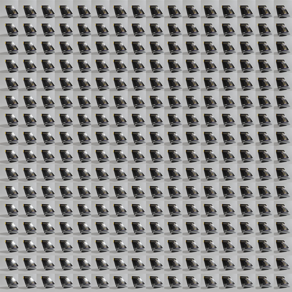
The images of all data cameras are generated in a 2D array of sub-images in a large image. The following image is an example output of a lightfield camera, rescaled to 1024x1024 resolution. The image is split to 16x16 camera array, where each square corresponds to a single data camera. The top-left sub-image corresponds to the top-left data camera in the camera array. Similarly, the top-left corner of the sub-image corresponds to the to-left corner of the data-camera's view.
To implement this you will need to write your own LightfieldCamera::GenerateRay()
function (overriding the base class's). Note that to get correct ray differentials at the boundary
between different data cameras you will also need to override
Camera::GenerateRayDifferential(). You do not need to implement any other function
defined in Camera.
Both of these functions take in a CameraSample and return a Ray and a
floating point weight for the ray to be used in the Monte Carlo estimation. In a pinhole camera
model, all rays are created equal (contribute equal weight to the Monte Carlo estimation) so we
can just return 1.0. The interesting part is generating the ray in the first place. The
CameraSample has three member variables: pFilm, which provides the
location of the sample on the film plane (if the film is [ x ]
pixels, the values will be on the range [0,)x[0,), with 0.5
corresponding to pixel centers). provides the location of the sample on the
lens in a parameterized uv space on the unit square; for a camera with a lens we'd
have to do an equal area transform so that this became a sample on the lens disk, but for pinhole
cameras the "lens" is a single point so this can be ignored. time provides the time
the ray is cast; this is useful if you have an animated scene; we do not, but pass this value
along to your ray anyways.
The origin of your ray will be at the camera's origin (the pinhole). You only need to calculate
the direction of the ray based on where it is on the film plane and your camera's field of view.
The pinhole camera section of PBRT 1.2.1, and the section on perspective cameras should help
significantly with your understanding; but as a recap, rays on the middle of the film plane
should come straight out of the camera; rays on the far edge of the film plane should make a
angle with the middle ray; the angle on the axis does
not depend on the coordinate and vice versa. It easiest to construct your ray in
camera space, and transform it using CameraToWorld afterwards.
For LightfieldCamera::GenerateRayDifferential() you will want to implement it so
that each data camera has the same ray differentials it would have had at the boundary if it
was a regular pinhole camera that was not sharing a film plane. The default implementation will
have massive incorrect jumps at data camera boundaries; see PBRT 6.1.
You will want to render the original settings for book.pbrt as soon as possible to
have a well-sampled light field to work with (it may take several hours to generate, so you'll
want to run it over night if possible), but for now turn down the resolution so there are only
8x8 data cameras with 128^2 resolution each, which should be 64x faster
to generate.
Step 3: Synthesize a Final Image from the LightField
In this step we will add an extra feature to imgtool command to synthesize an image
using the pre-rendered light field. You will need to modify the imgtool source code
at tools/imgtool.cpp to add the functionality.
We start with adding the new command to the usage string:
lightfield options:
    --camsperdim <x> <y>                    Number of data cameras in the X and
                                            Y direction, respectively
    --camerapos <x> <y> <z>                 Position of the desired camera for
                                            reconstruction (treating the data
                                            camera plane as z = 0)
    --filterwidth <fw>                      Width of the reconstruction filter (in
                                            meters on the camera plane)
    --focalplanez <fz>                      Z position of the focal plane for
                                            reconstruction (treating the data
                                            camera plane as z = 0)
    --griddim <xmin> <xmax> <ymin> <ymax>   The bounding box of the data cameras
                                            positions in the x and y dimensions
                                            (in meters)
    --inputfov <f>                          FOV (in degrees) of the input
                                            lightfield data cameras
    --outputfov <f>                         FOV (in degrees) of the output image
    --outputdim <w> <h>                     Output size in pixels per dimension
Modify the main() function to call the lightfield() function (which you
will be implementing) when the first command line argument is "lightfield". Here is a
skeleton of the lightfield function that parses the arguments specified in the usage string (without
much error handling!), reads the light field image (sometimes referred to as the ray database), and
saves an output image (without writing useful values to it):
int lightfield(int argc, char *argv[]) {

    const char *outfile = "resolvedLightfield.exr";
    Bounds2f griddim(Point2f(0, 0));
    float inputfov = 90.0f;
    float outputfov = 45.0f;
    Vector2i camerasPerDim(1, 1);
    Point2i outputDim(256, 256);
    float filterWidth = 0.05f;
    float focalPlaneZ = 10.0f;
    Point3f cameraPos(0,0,-0.02f);
    int i;
    for (i = 0; i < argc; ++i) {
        if (argv[i][0] != '-') break;
        if (!strcmp(argv[i], "--inputfov")) {
            ++i;
            inputfov = atof(argv[i]);
        } else if (!strcmp(argv[i], "--outputfov")) {
            ++i;
            outputfov = atof(argv[i]);
        } else if (!strcmp(argv[i], "--camsperdim")) {
            ++i;
            camerasPerDim.x = atoi(argv[i]);
            ++i;
            camerasPerDim.y = atoi(argv[i]);
        } else if (!strcmp(argv[i], "--outputdim")) {
            ++i;
            outputDim.x = atoi(argv[i]);
            ++i;
            outputDim.y = atoi(argv[i]);
        } else if (!strcmp(argv[i], "--camerapos")) {
            ++i;
            cameraPos.x = atof(argv[i]);
            ++i;
            cameraPos.y = atof(argv[i]);
            ++i;
            cameraPos.z = atof(argv[i]);
        } else if (!strcmp(argv[i], "--griddim")) {
            ++i;
            griddim.pMin.x = atof(argv[i]);
            ++i;
            griddim.pMax.x = atof(argv[i]);
            ++i;
            griddim.pMin.y = atof(argv[i]);
            ++i;
            griddim.pMax.y = atof(argv[i]);
        } else if (!strcmp(argv[i], "--filterwidth")) {
            ++i;
            filterWidth = atof(argv[i]);
        }  else if (!strcmp(argv[i], "--focalplanez")) {
            ++i;
            focalPlaneZ = atof(argv[i]);
        } else {
            usage();
        }
    }
    if (i + 1 >= argc)
        usage("missing second filename for \"lightfield\"");
    else if (i >= argc)
        usage("missing filenames for \"lightfield\"");

    const char *inFilename = argv[i], *outFilename = argv[i + 1];
    Point2i res;
    std::unique_ptr image(ReadImage(inFilename, &res;));
    if (!image) {
        fprintf(stderr, "%s: unable to read image\n", inFilename);
        return 1;
    }

    std::unique_ptr outputImage(new RGBSpectrum[outputDim.x*outputDim.y]);

    // Render from your lightfield here...

    WriteImage(outFilename, (Float *)outputImage.get(), Bounds2i(Point2i(0, 0), outputDim),
        outputDim);
    return 0;
}
When you run imgtool, "camsperdim", "griddim", and
"inputfov" should match the values used to generate the light field image in the first
place. "outputdim" defines the size of the output image, "camerapos"
positions the synthetic camera, "outputfov" sets up the field of view of the output camera, and "focalplanez" defines the focal plane for the synthetic
camera. We will be using the phenomenological model laid out in
Dynamically Reparameterized Light Fields
for reconstruction in this section: "filterwidth" implicitly controls the effective
aperture size of the synthetic camera in this model; but we will be revisiting this approach in a
later section of the assignment. The desired camera is assumed to have the same rotation as the data
cameras, pointing down their Z axis with the same up vector they have.
Note that the input light field and output image are stored in a flat array of
RGBSpectrum. These images are stored in row-major order (all the pixels of the first
row are first, then all pixels of the second row, etc). RGBSpectrum wraps up RGB
values used to store radiance/irradiance/sensor response; RGBSpectrums has defined
multiplication by a Float, so you never need to actually grab the values out to
implement things like a weighted average of radiances.
Recall from class that evaluating the response of a camera involves solving a five dimensional integral; 2 dimensions for the sensor's pixel area, 2 dimensions for the directions of incoming light, and 1 dimension for time. For now, we will be assuming that the light field image is capturing a particular moment in time, and the synthetic camera we are rendering to is static; this removes the time dimension from the integral. For this section only, we will ignore the 2 dimensions of pixel area for the synthetic camera sensor, evaluating only the light incident on the pixel's center.
This leaves the two dimensions corresponding to the incoming light direction. Instead of solving this using a Monte Carlo estimator, Dynamically Reparameterized Light Fields approximates this integral by evaluating a weighted average of individual rays in several data cameras. Recall that our ray database is a finite discrete sampling of the 4D light field; since the space of rays is continuous, that means the probability that we have that exact ray in the light field image is 0. If we want to sample a ray (say to get the value for a pixel of the output image using the desired camera), we need to interpolate the ray from "nearby" rays in the ray database.
For this section we will use a three step procedure to reconstruct the ray. First, we will find where the ray intersects the data camera plane (at coordinates ) and the focal plane (at coordinates ). Then we will find all data cameras within the filter radius of ; and take a weighted sum of the radiance values stored in the ray database for all rays leaving said data cameras and intersecting . This is illustrated in figure 4 of the paper (in our case F-plane and C-plane are parallel since we do not have camera rotations.):
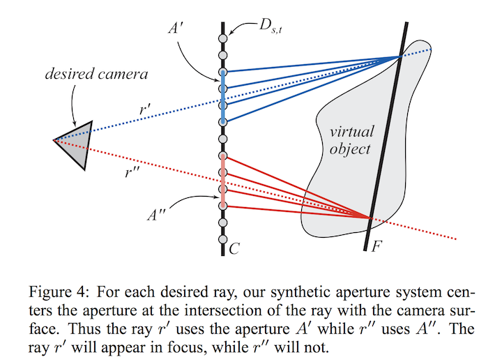
Notice that this is a weighted sum of rays that focus on the same point as the initial ray; they are samples that could have been drawn to evaluate irradiance if we were doing Monte Carlo integration of the irradiance and our lens subtended the same area as our filter. That is precisely the approximation we are making (along with our ad-hoc weights; consider why this is a biased approximation); this is a phenomenological approach; it reproduces the effect of defocus blur but is not physically correct.
There are two unanswered questions in how to implement the above approach:
- When sampling a ray from a data camera, how to interpolate from existing rays? First compute the coordinate in the image corresponding to the ray, then use bilinear interpolation (see pbrt 10.3.4) to interpolate the ray value from its four closest neighbors in the subset of the ray database corresponding to the data camera.
- What weights to use for the weighted average of the rays from each data camera? Use a cone filter (weight falls off linearly with distance from the filter's center), just make sure to normalize the weights so that they add up to one (this is easiest by summing the weights and dividing the result by this weight sum).
Once you have correctly implemented this section, you should be able to run:
Change the settings (while keeping the filter width roughly the same) so that the author's names are well focused and generate an image to submit.
Step 4: A Monte Carlo Approach
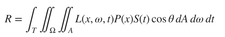
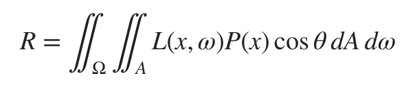
In step 3 we leverage the work of Isaksen et. al to quickly generate plausible final renderings from the light field. To do so, we gave up accurate modelling of the desired camera to have an easily formulated algorithm for generating final pixel values. In this step, we will instead perform Monte Carlo integration to solve the camera equation:
The only primitive operation we need from the light field to solve this equation is a mapping form a ray to . In step 3, we freely combined the solid angle integration with this mapping. In this step we will instead attempt to isolate the mapping and let Monte Carlo integration take care of the rest.
We can reuse most of our infrastructure from Step 3. We can still find rays in the data cameras using the same approach., but we will interpolate the final rays from the data camera rays using bilinear interpolation. This drastically decreases the size of our reconstruction filter and gives us a more plausible estimate of the radiance coming in along a single ray.
Now we can mimic any camera/film setup in pbrt by "tracing" rays the same way in
this light field as we would have in the original scene; with the difference that no actual
tracing happens in the light field, and we just look up the ray in the ray database using two-stage
bilinear interpolation.
Add these parameters to your imgtool lightfield usage instructions:
--montecarlo                        If this flag is passed, use Monte Carlo
                                    integration generate the final image
                                    (this renders filterwidth useless)
--lensradius <r>                    The radius of the thin lens in the
                                    thin lens approximation for the output
                                    camera.
--samplesperpixel <p>               The number of samples to take (per pixel)
                                    in Monte Carlo the integration of the
                                    final image.
They should have the following defaults:
bool monteCarlo = false;
        float lensRadius = 0.0f;
        int samplesPerPixel = 1;
and here is some argument parsing code (to add into the parsing code in Step 3) you can add if you do not want to write it from scratch:
if (!strcmp(argv[i], "--montecarlo")) {
      monteCarlo = true;
  } else if (!strcmp(argv[i], "--lensradius")) {
      ++i;
      lensRadius = atof(argv[i]);
  }  else if (!strcmp(argv[i], "--samplesperpixel")) {
      ++i;
      samplesPerPixel = atoi(argv[i]);
  }
Note that the focal plane is specified relative to the data camera plane, not the desired camera. Once you have the parameters all set, you can perform Monte Carlo integration of the integral:
For this assignment, we assume a static scene and camera, so the time integral goes away:
We can solve this integral using a Monte Carlo estimator that samples rays whose origins are
sampled from the sensor area and whose directions are sampled from all directions that hit the
lens. We will be using the thin lens approximation (detailed in pbrt 6.2.3 and in lecture, and
implemented in perspective.cpp for pbrt's perspective camera). We will follow pbrt and simplify our
Monte Carlo estimator; throwing out the cosine term and weight from the solid angle integration
integration (the thin lens model already used a paraxial approximation, which threw this exactness
out the window).
Our estimator will reduce to simple average of radiance values for rays sampled in the method
defined by pbrt 6.2.3 per pixel. In order to do Monte Carlo integration you will need to be able to
generate random numbers (see the RNG class) and transform a sampling of the unit square
to a sampling of the unit disk (for the lens); you will be sampling random points on the sensor
pixel and random points on the lens for every ray in the estimator. See
ConcentricSampleDisk().
Reproduce your final image from Step 3 using your newly implemented Monte Carlo method. It will necessarily be slightly different since we are now using a more accurate approximation. Make sure to keep track of the command lines you use to generate each image.
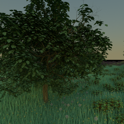
Download the ecosys scene. There is already a light field rendered (it
took ~10 hours to render on a mid-range desktop) in ecosys_lightfield.exr. The light
field image is at 8192x8192 resolution with 64 samples per pixel; and the camera
settings were:
Camera "lightfield"
      "float fov" [ 60 ] "integer camerasperdim" [16 16]
      "float cameragridbounds" [-2.5 2.5 -1.5 1.5]
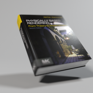
All other settings were identical to those in ecosys.pbrt. The following picture shows
one of the data camera images from ecosys_lightfield.exr.
Render and image using the thin-lens camera specified in ecosys.pbrt. Render an
image using the same camera parameters from the ecosys_lightfield.exr instead. You
can select the samples per pixel, so long as the two images are roughly comparable. These images
both demonstrate an interesting effect: with a wide enough lens, and by focusing on the far
hilside, we can effectively "see through" the trees. Explain why this happens and describe the
difference between the two images.
Produce two other images by moving the camera and focal plane to focus on the two trees (one tree per image!) visible in the light field (and in the original image). You may narrow the lens radius but make sure it is above zero. Feel free to generate new light fields with higher or lower angular resolution, spatial resolution, spatial separation, or samples per pixel if it improves your results. You will almost certainly have noticeable visual artifacts in your images; that is fine, but provide an explanation for why they exist, how you mitigated them, and how you would alleviate them given more time to generate the light field.
Step 5: Optional Bonuses
There are several interesting extensions you can make to this project. You may choose one of the
below, augment your imgtool implementation, and document what you have done. Produce
at least two distinct images:
- Impossible Focal Surfaces: Since we are synthesizing from a captured light field, we are not limited to physically-realizable camera systems for image generation. For example, you could tilt the focal plane, or make it some non-planar suface.
- Realistic Camera Rendering: Use the infrastructure from Part 4, but instead of emulating a
thin-lens perspective camera, implement a realistic camera (following pbrt 6.4). The easiest
way to impement this is to actually instantiate a
RealisticCameraand call itsGenerateRay(); which provides both the ray and the weight to use in the Monte Carlo estimator.
Step 6: Short Discussions
- How would you modify the approach in step 4 (and the implementation of LightField camera) to support the time dimension of the camera integral?
- What happens to the images you generate if your lightfield is undersampled (the number of camera per dimension is small)? Why?
- What happens to your final images if you seek to fix the artifacts described in the previous question by using many cameras but with very low resolution (say a 128x128 grid of 64x64 resolution cameras)?
HINTS
SUBMISSION
To submit your work, create a.zip or .tar.gz file that contains:
- All the code files you added and/or modified in pbrt (
api.cpp,lightfield.h,lightfield.cpp, andimgtool.cpp). - The new images (and their correspanding imgtool command lines) you created in Steps 3-5.
- The description of the difference between the two images generated with the same camera (one with the light field and one directly from the scene) in Step 4, and the descriptions specified about the visual artifacts in the other images in Step 4.
- Any new or modified scene files from Step 4 or (the optional) Step 5.
- The answers from step 6.
- A description of troubles you ran into during implementation, and how you overcame or worked around them.