Lab 4
Sampling Efficiency
Due: Thursday, January 15th, 2018, 23:55
This lab was modeled after the assignment 4 of Stanford's Image Synthesis class.- Individual Effort:
- No team participation is really encouraged in the case of the homework or the labs.
Objectives
In this assignment you will evaluate the efficiency of different sampling strategies for Monte-Carlo integration. While there is very little coding in this assignment, you will probably need to script pbrt to collect the right data. The data collection itself may take some time, so plan ahead to make sure you have time to complete rendering. You can download the necessary scene files and reference images.
Sampling and Variance
Variance of a random variable is defined as . To compute the variance of an image rendered by pbrt we can compare it, pixel by pixel, to a reference image that we consider to be ground truth for . We've included three EXR images that will serve as ground truth for this assignment (quads_groundtruth.exr, quads_zoom_groundtruth.exr, and frame25_groundtruth.exr). These
scenes were rendered with 16384 samples per pixel to ensure that they are very close to the correct image. To measure
the variance of any image you render, you can use the imgtool program that you modified in
Lab 3:
imgtool diff image_ref.exr yourimage.exrThis will print something like:
  Images differ: 297985 big (98.54%), 301493 small (99.70%)
  avg 1 = 0.0617386, avg2 = 0.0156974 (293.304010% delta)
  MSE = 0.0060754, RMS = 7.794%
Look at the code for
imgtool and convince yourself that the MSE (mean-squared error) value it calculates is
equivalent to the variance. You may need to modify imgtool to ensure it always prints the MSE value
regardless of how close the two images are.
As we increase the number of samples taken, we expect the the variance to go down. We will measure this change
empirically by modifying the pixelsamples variable in the scene files. The file quads.pbrt contains a
scene with a single area-light, a square occluder, and a large ground plane:
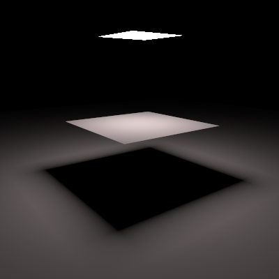
Render this scene varying the number of samples from 1 to 1024, and compute the variance of each image. You only need to measure square powers of 2 (i.e. 1, 4, 16, 64, 256, 1024) since many of the samplers in pbrt will round this number to a power of 2 per dimension anyway.
The scene file is setup to use a uniform random sampler. Let's compare this to a stratified random sampler, and a
sampler that uses the low-discrepancy Halton sequence, by changing the Sampler and finding the variance
for each image.
Deliverables
First, submit a graph showing the variance for the random, stratified, and low-discrepancy samplers as you increase pixelsamples from 1 to 1024 for thequads.pbrt scene. You will probably want to use log scale for
both axes since you are only considering powers of 2. Furthermore, you should answer the following questions:
Question 1. When using Monte-Carlo sampling with uniformly sampled random variables, how does the variance change as a function of the number of samples taken, ? Does the data you collected reflect this behavior?
Question 2. How does the Halton sequence sampler perform in comparison to random sampling? Why does distributing the samples evenly through space change the variance in comparison to random sampling?
Question 3.How does the stratified sampler perform in comparison to the other sampling methods?
Stratified Light Sampling
The "directlighting" Integrator, by default, shoots one shadow ray to each light source for every sample
per pixel. If you have 10 lights and 32 samples per pixel, this will result in 32 primary visibility rays per pixel
and 320 shadow rays per pixel. This is in contrast to the standard path tracing Integrator, which always evaluates
one path per sample. But using this we can simulate stratified sampling on just the area light on both
quad.pbrt and quads_zoom.pbrt (which is the same scene, just with a different camera) scene.
Create new variants of the scenes so that the one square area light is broken up into 16 square area lights arranged
in a 4x4 grid covering the same area as the original area light (and using the same power). By rendering lots of
samples, these new versions of the scenes should converge to the same image as the old versions. Note that there is no
quad primitive; squares are represented as two triangles, and pbrt treats each triangle as two separate lights, so your
new scenes will cast 32 shadow rays per pixel sample (and the original scenes will cast 2 shadow rays per pixel sample).

Render the new scene variants with 4 samples/pixel, and the original scene variants with 64 samples/pixel (all using
the "random" Sampler). All of these images should use 128 shadow rays per pixel. We'll compare their
variances and where the errors appear in both version.
Deliverables
Report the variances for the two variants of each of the two scenes in a (2x2) table. Provide "diff"
images of these four scene variants (use the --outfile parameter of the imgtool diff tool
to create the diff image with respect to the ground truth.
Make sure to update pbrt to the latest version from git, only recent versions have fixed saving the diff images).
Answer the following question:
Question 1. Which of the two scenes sees the most drastic improvement when switching to the stratified light sampling strategy? Why?
Importance Sampling Efficiency
We also discussed two important concepts that we will explore here: importance sampling and efficiency.
Before we begin, take a look at the ground truth image for measure-one/frame_25.pbrt (below), and if
you'd like, the original video it was used in: ZERO-DAY.
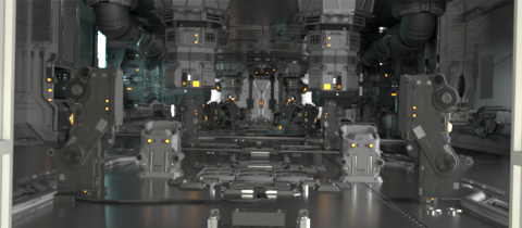
We demonstrated we could drastically improve convergence of the radiance integral by evaluating the hemispherical reflectance integral at a point by directly sampling an area light source, instead of sampling the entire hemisphere of directions. This is a type of importance sampling: when evaluating direct illumination at a point we know the result will be zero in all directions besides those going to the light source.
This scene contains over 8,000 area lights. If we want to sample light sources instead of the entire hemisphere of directions, we need to choose some probability distribution of which lights to sample for our importance-sampled Monte Carlo estimator (this wasn't an issue in the quad scene with only one light, we trivially chose to sample from the only light source with probability 1).
pbrt has three built-in methods for choosing light sources when evaluating direct illumination (which you can choose
by altering the "lightsamplestrategy" in the .pbrt file):
"uniform", "power", and "spatial":
- "
uniform" samples all light sources uniformly, - "
power" samples light sources according to their emitted power, - "
spatial" computes light contributions in regions of the scene and samples from a related distribution.
spatial" is somewhat involved, but basically the scene is broken up into
voxels (roughly cubic volumes); the amount of light coming into each voxel from each light is sampled (at 128
quasi-random points within the voxel, with no visibility calculations), and a probability distribution over lights,
where the probability of sampling a light is proportional to the amount of light contributed to each voxel (with
some non-zero minimum), is created for each voxel.
Compute the variance and efficiency for the measure-one/frame_25.pbrt scene and the original quad
scene using all three approaches at 512 samples/pixel (use the "random" Sampler).
Estimate the number of samples you would require to get the same quality as the "spatial" result
using "uniform" and "power".
Deliverables
You should provide the variance and efficiency numbers you calculated for each approach; beside answering the following questions:
Question 1. How long would it take to render an equal-to-spatial quality version of the image using the
"uniform" strategy? How about using the "power" strategy?
Question 2. Describe a scene where the "power" strategy would be significantly worse than the
"uniform" strategy.
Question 3. Describe a scene where the "spatial" strategy would be significantly worse than the
"power" strategy.
Bonus
See if you can improve the efficiency of the "spatial" light sampling approach by taking into account
visibility in some way. There's even a TODO directly in the code about it; see
SpatialLightDistribution::ComputeDistribution() in lightdistrib.cpp.
Submit a brief description of your approach, the measured improvement in efficiency on the
measure-one/frame_25.pbrt scene, and the code you changed for up to 1 bonus point.
Submission
Please submit your answers in a single PDF file in moodle, in Lab4 section
here.
If you have multiple files to upload (e.g. source code or supplementary pictures),
please upload all your submission as a single compressed ZIP file.
We expect a good student to have to work approximately 14 hours on this assignment.
Include one paragraph about your estimated effort you put into this lab. How many (focused) hours of work did it take you and roughly where did you spend most of your time.